Understanding regularising energies

Context

In our generatives models, images are often assumed to stem from a multivariate Gaussian distribution, where the number of dimension is equal to the number of pixels or voxels in the image. In a Bayesian context, finding the optimal (deformation, velocity, probability, …) field $\mathbf{y}$ given an observed image $\mathbf{x}$ consists of optimising the log probability:

$\begin{split}\hat{\mathbf{y}} & = \arg\!\max_{\mathbf{y}} \overbrace{\ln p(\mathbf{x} \mid \mathbf{y})}^{\mathrm{similarity}} + \overbrace{\ln \mathcal{N}\left(\mathbf{y} \mid \mathbf{0}, \mathbf{L}^{-1}\right)}^{\mathrm{regularisation}} \\ & = \arg\!\min_{\mathbf{y}} -\ln p(\mathbf{x} \mid \mathbf{y}) + \frac{1}{2}\mathbf{y}^{\mathrm{T}}\mathbf{L}\mathbf{y}\end{split}$

It is useful to parameterise this multivariate Gaussian so that it corresponds to the belief we can have about the image appearance. Whether we are interested in bias fields, deformation fields or tissue probability maps, a common assumption is that images are smooth, i.e., they do not show sharp edges and vary slowly. A way of enforcing such smoothness is by defining precision matrices ($\mathbf{L}$) based on differential operators, so that the regularisation term penalises spatial derivatives – i.e., gradients – of the image.

Typically, assume that a matrix $\mathbf{K}$ allows to compute gradients of an image by using finite differences, i.e., $\mathbf{K}\mathbf{y}$ returns the first derivatives of $\mathbf{y}$. Then $(\mathbf{K}\mathbf{y})^{\mathrm{T}}(\mathbf{K}\mathbf{y}) = \mathbf{y}^{\mathrm{T}}\mathbf{K}^{\mathrm{T}}\mathbf{K}\mathbf{y}$ returns the sum of square gradients of $\mathbf{y}$. We recognise the regularisation term in the previous objective function, with $\mathbf{L} = \mathbf{K}^{\mathrm{T}}\mathbf{K}$, which is positive-definite by construction.

In this article, we describe a selection of regularisation “energies” used in SPM, which were presented in Ashburner (2007). We provide their continuous and discrete form, show the equivalent sparse matrices and generate random samples from the corresponding Gaussian distributions. All examples use displacement fields, i.e., images with several components (2 for 2D images, 3 for 3D images). They are color coded, so that all components can be seen at once, according to the following scale:

**Figure 1.** Color coding of displacements.

Absolute values

A first basic penalty can be placed on the image absolute values. This is not a “smooth” regularisation but it can be useful to avoid very unlikely values. When working with log-probability images (e.g., tissue probability maps), it can be seen as a Dirichlet prior. When working with diffeomorphisms, it ensures that the complete transform can be recovered with a reasonably low number of integration steps.

On a two-dimensional continuous space, the corresponding energy is:

$\mathcal{E} = \frac{\lambda}{2} \int_\Omega v_x(\mathbf{x})^2 + v_y(\mathbf{x})^2 \mathrm{d}\mathbf{x}$

Formally, for discrete images, it is equivalent to saying that $\mathbf{L} = \lambda\mathbf{I}$. The corresponding precision matrix (for deformation fields defined on a 1mm isotropic 5x5 lattice, with $\lambda = 1$) is:

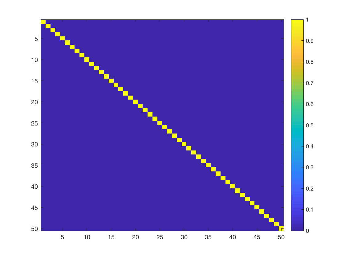
Precision matrix for the absolute value penalty. — **Figure 2.** Precision matrix corresponding to a penalty on squared values.

Here are four samples obtained from prior distributions with a varying $\lambda$ (10¹, 10², 10³, 10⁴). Note that the displacement magnitude (in the top left corner) varies accordingly:

Four random samples from the absolute distribution. — **Figure 3.** Random samples obtained with an increasing penalty on absolute displacements.

Membrane energy

A first way of encouraging smoothness is by penalising the squares of the fist derivatives. It is a very local penalty that often results in images with blobs of intensities. On a two-dimensional continuous space, the corresponding energy is:

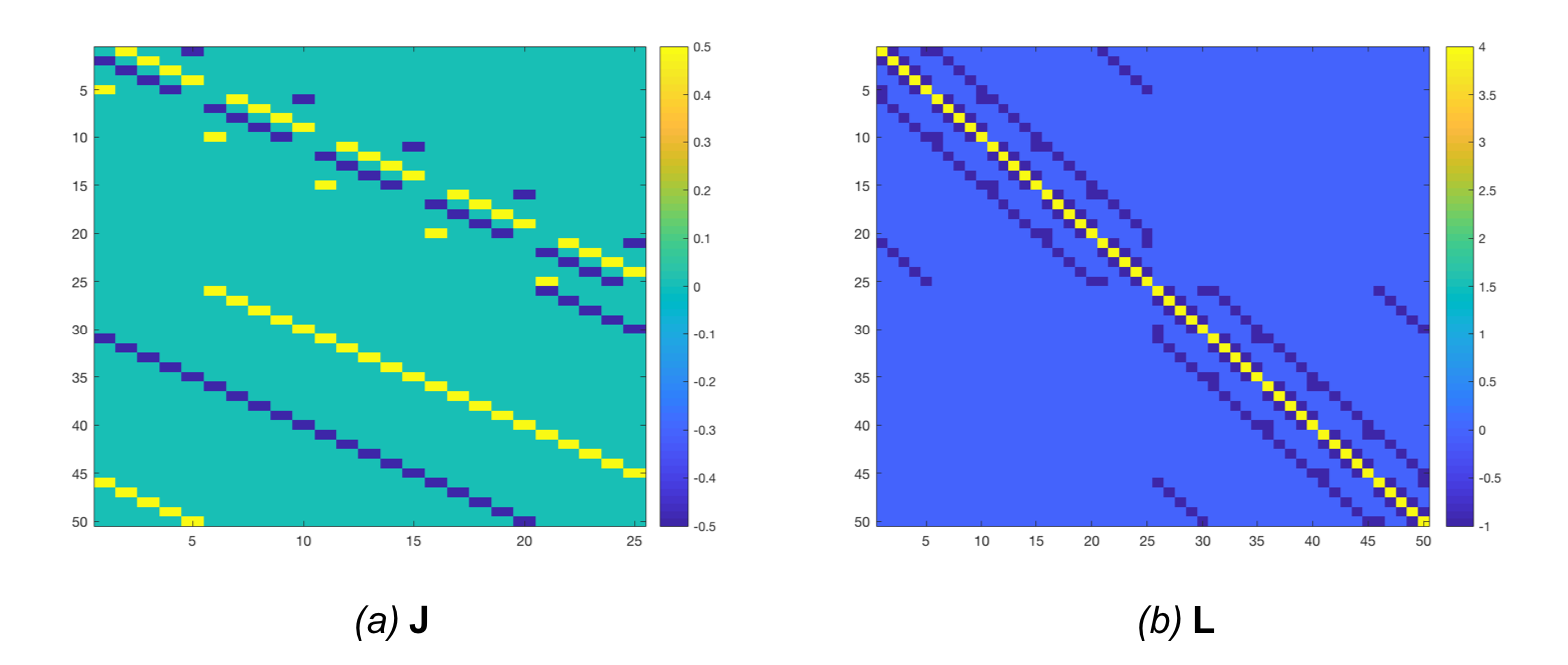
$\mathcal{E} = \frac{\lambda}{2} \int_\Omega \left[\frac{\partial v_x}{\partial x}(\mathbf{x})\right]^2 + \left[\frac{\partial v_x}{\partial y}(\mathbf{x})\right]^2 + \left[\frac{\partial v_y}{\partial x}(\mathbf{x})\right]^2 + \left[\frac{\partial v_y}{\partial y}(\mathbf{x})\right]^2 \mathrm{d}\mathbf{x}$

For discrete images, this can be obtained by building a matrix $\mathbf{J}$ that computes all possible first order finite differences. Such a matrix is shown in Figure 4.a for a 2D 5x5 input. We then multiply it with its transpose ($\mathbf{L} = \mathbf{J}^{\mathrm{T}}\mathbf{J}$), so that $\mathbf{v}^{\mathrm{T}}\mathbf{L}\mathbf{v}$ returns the sum of square finite differences. This matrix is shown in Figure 4.b.

Sparse Jacobian matrix and precision matrix for the membrane energy. — **Figure 4.** (a) Sparse matrix that allows computing Jacobians. (b) Precision matrix corresponding to a penalty on squared first derivatives.

Below are four samples obtained from prior distributions with a varying $\lambda$ (10¹, 10², 10³, 10⁴)¹:

Four random samples from the membrane distribution. — **Figure 5.** Random samples obtained with an increasing penalty on first derivatives.

Bending energy

Penalising second derivatives makes the regularisation less local. This is what we often think as smoothness in the sense that the “slope” in the image can be steep but varies slowly. On a two-dimensional continuous space, the corresponding energy is:

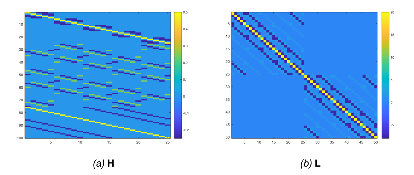
$\mathcal{E} = \frac{\lambda}{2} \int_\Omega \left[\frac{\partial^2 v_x}{\partial x^2}(\mathbf{x})\right]^2 + \left[\frac{\partial^2 v_y}{\partial y^2}(\mathbf{x})\right]^2 + 2\left[\frac{\partial^2 v_x}{\partial x \partial y}(\mathbf{x})\right]^2 + 2\left[\frac{\partial^2 v_y}{\partial x \partial y}(\mathbf{x})\right]^2 \mathrm{d}\mathbf{x}$

For discrete images, this can be obtained by building a matrix that computes all possible second order finite differences. Such a matrix is shown in Figure 6.a for a 2D 5x5 input. We then multiply it with its transpose ($\mathbf{L} = \mathbf{H}^{\mathrm{T}}\mathbf{H}$), so that $\mathbf{v}^{\mathrm{T}}\mathbf{L}\mathbf{v}$ returns the sum of square finite differences. This matrix is shown in Figure 6.b.

Sparse Hessian matrix and precision matrix for the bending energy. — **Figure 6.** (a) Sparse matrix that allows computing Hessians. (b) Precision matrix corresponding to a penalty on squared second derivatives.

Here are four samples obtained from prior distributions with a varying $\lambda$ (10¹, 10², 10³, 10⁴)¹:

Four random samples from the bending distribution. — **Figure 7.** Random samples obtained with an increasing penalty on second derivatives.

Membrane + Bending

Combining both regularisations encourages smooth and flat slopes as illustrated by these random samples:

Linear-Elastic energy

The membrane and bending energies allow to control the magnitude and smoothness of the image slope. When dealing with deformations, it might be interesting to include additional prior beliefs about the local geometry of the deformation, i.e., the amount of zooms (or volume change) and shears that it embeds. The linear elastic energy is based on two terms: the first one penalises the symmetric part of the Jacobian (shears), while the other one penalises the divergence (zooms) of the deformation.

Symmetric part of the Jacobian (Shears)

On the continuum, this part of the energy can be written as:

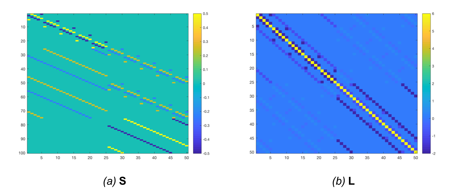
$\mathcal{E} = \frac{\mu}{2} \int_\Omega \frac{1}{2}\left[\frac{\partial v_x}{\partial y}(\mathbf{x}) + \frac{\partial v_y}{\partial x}(\mathbf{x})\right]^2 \mathrm{d}\mathbf{x}$

In discrete form, it can be obtained by multiplying the sparse “Jacobian operator” matrix used for the membrane energy with a “symmetric operator” matrix that, in each point, sums together the Jacobian and its transpose. The “symmetric Jacobian operator” matrix is shown in Figure 9.a, and the corresponding precision matrix is shown in Figure 9.b.

Sparse Hessian matrix and precision matrix for the linear-elastic (symjac) energy. — **Figure 9.** (a) Sparse matrix that allows computing the symmetric part of the Jacobian. (b) Precision matrix corresponding to a penalty on the linear-elastic energy's first component (shears).

As before, four samples were obtained from prior distributions with a varying $\lambda$ (10¹, 10², 10³, 10⁴)¹:

Four random samples from the linear-elastic (symjac) distribution. — **Figure 10.** Random samples obtained with an increasing penalty on shears.

Divergence (zooms)

On the continuum, this part of the energy can be written as:

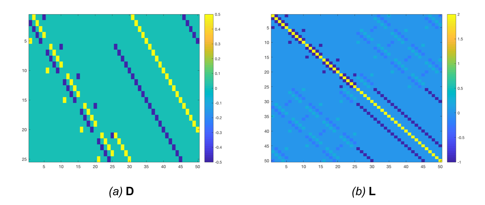
$\mathcal{E} = \frac{\mu}{2} \int_\Omega \left[\frac{\partial v_x}{\partial x}(\mathbf{x})\right]\left[\frac{\partial v_y}{\partial y}(\mathbf{x})\right] \mathrm{d}\mathbf{x}$

In discrete form, it can be obtained by “aligning” matrices that allows computing the gradient along each direction. The “divergence operator” matrix is shown in Figure 11.a, and the corresponding precision matrix is shown in Figure 11.b.

Sparse Hessian matrix and precision matrix for the linear-elastic (div) energy. — **Figure 11.** (a) Sparse matrix that allows computing the divergence. (b) Precision matrix corresponding to a penalty on the linear-elastic energy's second component (zooms).

Here are four samples obtained from prior distributions with a varying $\lambda$ (10¹, 10², 10³, 10⁴)¹:

This term penalises a very particular feature, the volume, without promoting smoothness. Images generated from this distribution can be compared to Rubik’s cubes: they can be sheared at will but the volume of the cube is always preserved.

Linear-Elastic

Obviously, it doesn’t make sense using each component separately. Here are samples generated from the combined linear-elastic distribution:

Boundary conditions

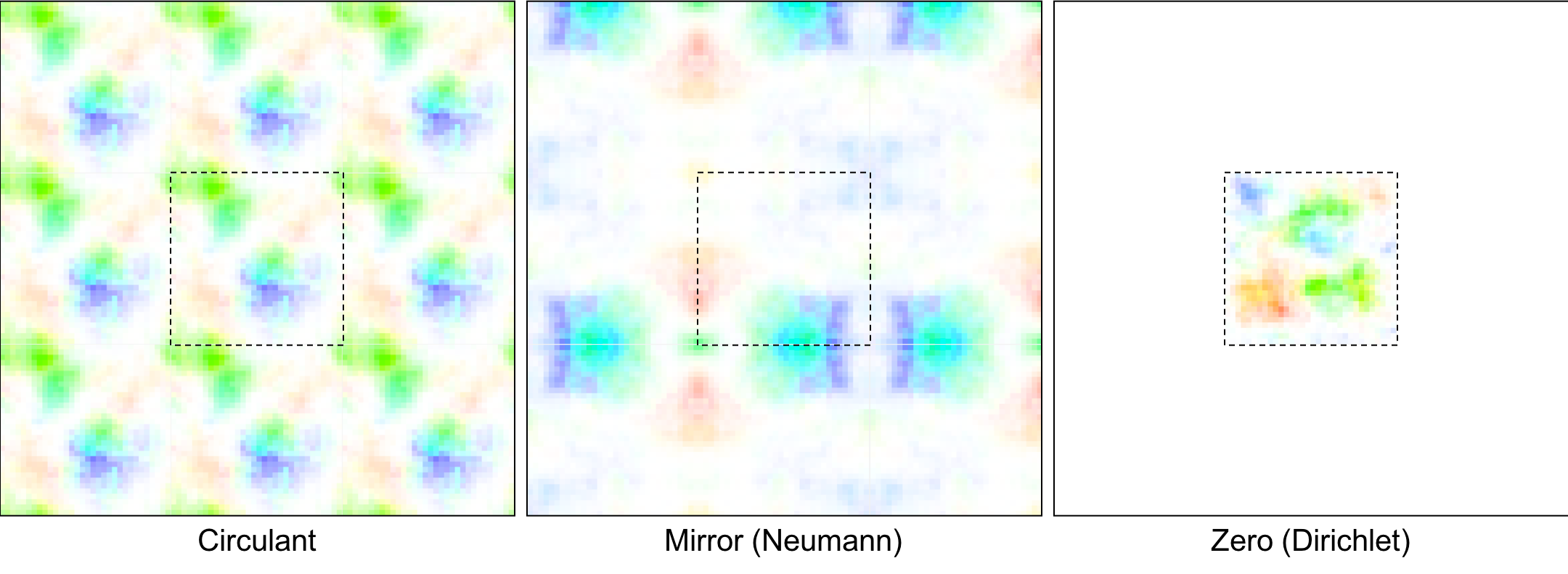
All these energies are based on spatial derivatives, which must be computed at any point, even next to the edges of the field of view. There are different ways of dealing with derivatives at the boundary, which change greatly the range of possible fields:

Circulant boundary conditions are based on the idea that the left and right edges are the same (the bottom and top edges, too, as well as any opposite edges). As such, the most left voxel is a neighbour of the most right one, and the image can be seen as wrapping around the boundaries. This means that, to be likeliy, these voxels must have similar values.
Neumann boundary conditions force first-order spatial derivatives to be zero at the boundary. This is obtained by assuming that the image is “mirrored” around the edges.
Dirichlet boundary conditons force the field values to be zero at the boundary. This is obtained by assuming voxels outside of the field of view to be zero.

Those three conditions are illustrated in the figure below. Three random samples (within dotted edges) are shown, each with different boundary conditions. The “virtual” values outside of the field of view are also shown (within solid edges).

**Figure 14.** Three random samples with different boundary conditions. Voxel values outside of the field of view are also shown.

Created by Yaël Balbastre on 3 April 2018. Last edited on 20 April 2018.

A small penalty was added on absolute values to make the precision matrix well conditioned. ↩ ↩² ↩³ ↩⁴

Computational Anatomy notes