Gamma

Ususal parameterisation

Probability distribution function

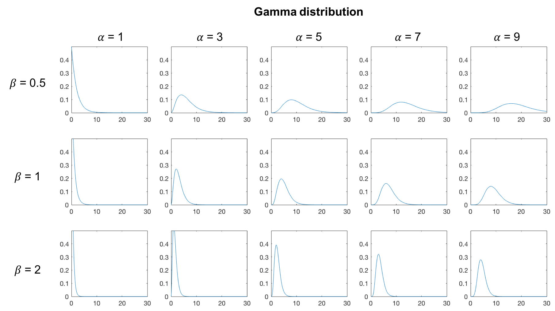
The Gamma distribution is defined on $\left[0, \infty\right[$. There are two usual parameterisation:

• This first one is $(\alpha, \beta)$ where $\alpha$ is called the shape parameter and $\beta$ the rate parameter.

$$\begin{align*} \mathcal{G}\left(x \mid \alpha, \beta\right) & = \frac{\beta^\alpha}{\Gamma(\alpha)}x^{\alpha-1}\exp(-\beta x) \\ \ln\mathcal{G}\left(x \mid \alpha, \beta\right) & = \alpha\ln\beta - \ln\Gamma(\alpha) + (\alpha-1)\ln x - \beta x \\ \mathbb{E}\left[x\right] & = \frac{\alpha}{\beta} \\ \mathbb{E}\left[\ln x\right] & = \psi(\alpha) - \ln\beta \\ \mathbb{V}\left[x\right] & = \frac{\alpha}{\beta^2} \\ \mathbb{V}\left[\ln x\right] & = \psi_1(\alpha) \end{align*}$$

where $\Gamma$ is the Gamma function^[wiki], $\psi$ is the digamma function^[wiki] and $\psi_1$ is the trigamma function^[wiki].

The distribution has a mode only if $\alpha \geqslant 1$:

$$\max_x \mathcal{G}\left(x \mid \alpha, \beta\right) = \frac{\alpha-1}{\beta}$$

• A second parameterisation is $(k, \theta)$, where $k = \alpha$ is the shape parameter and $\theta = \beta^{-1}$ is the scale parameter. The PDF, mean and variance can be easily obtained from the above formulas by substitution.

Maximum likelihood estimators

Let $\mathbf{x} = (x_n)$ a set of observed realisations from a Gamma distribution.

$\hat{\beta} \mid \mathbf{x}, \alpha$	$= \frac{\alpha}{\overline{x}}$
$\hat{\alpha} \mid \mathbf{x}$	solution of: $\ln \hat{\alpha} - \psi(\hat{\alpha}) = \ln \overline{x} - \overline{\ln x}$
$\hat{\beta} \mid \mathbf{x}$	$= \hat{\beta} \mid \mathbf{x}, \hat{\alpha} = \frac{\hat{\alpha}}{\overline{x}}$

There is no closed form solution for $\hat{\alpha}$, but an approximate solution can be found by numerical optimisation.

Conjugate prior

We list here the distributions that can be used as conjugate prior for the parameters of an univariate Normal distribution:

$\beta \mid \alpha$

Gamma

$\mathcal{G}_\alpha$

Update equations can be found in the Conjugate prior article.

Kullback-Leibler divergence

The KL-divergence can be written as

$$\begin{align*} \mathrm{KL}\left(q \middle\| p\right) & = \mathbb{E}_q\left[\ln q(x)\right] - \mathbb{E}_q\left[\ln p(x)\right] \\ & = H\left(q, p\right) - H\left(q\right) \end{align*}$$

where $H$ is the cross-entropy. We have

$$\begin{align*} H\left(\alpha_1, \beta_1 \middle\| \alpha_0, \beta_0\right) & = -\alpha_0\ln\beta_0 + \ln\Gamma(\alpha_0) - (\alpha_0-1)\left(\psi(\alpha_1) - \ln\beta_1\right) + \alpha_1\frac{\beta_0}{\beta_1} \\ H\left(\alpha_1, \beta_1\right) & = -\ln\beta_1 + \alpha_1 + \ln\Gamma(\alpha_1) - (\alpha_1-1)\psi(\alpha_1) \end{align*}$$

Consequently

$$\boxed{\begin{split} \mathrm{KL}\left(\alpha_1, \beta_1 \middle\| \alpha_0, \beta_0\right) = & -\alpha_0\ln\frac{\beta_0}{\beta_1} + \alpha_1\left(\frac{\beta_0}{\beta_1} - 1\right) \\ & + \ln\Gamma(\alpha_0) - \ln\Gamma(\alpha_1) + (\alpha_1-\alpha_0)\psi(\alpha_1)\end{split}}$$

Related distributions

Specialisation
Exponential	$\mathrm{Exp}(\lambda) = \mathcal{G}(1, \lambda)$
Chi-squared	$\chi^2(\nu) = \mathcal{G}_\mathcal{N}(1, \nu) = \mathcal{G}\left(\frac{\nu}{2}, \frac{1}{2}\right)$
Generalisation
Generalised Gamma	$\mathcal{G}(\alpha, \beta) = \mathcal{G}^{(1)}(\alpha, \beta)$	q = 1
Wishart	$\mathcal{G}_\mathcal{N}(\lambda, n) = \mathcal{W}_1(\lambda, n)$	K = 1
Generalised Integer Gamma
Generalised Inverse-Gaussian
Power
Inverse-Gamma	$x \sim \mathcal{G}(\alpha, \beta) \Rightarrow \frac{1}{x} \sim \mathrm{Inv-}\mathcal{G}\left(\alpha, \frac{1}{\beta}\right)$
Generalised Gamma	$x \sim \mathcal{G}(\alpha, \beta) \Rightarrow x^q \sim \mathcal{G}^{\left(1/q\right)}\left(\frac{\alpha}{q}, \beta^q\right)$	q > 0

Univariate Normal precision conjugate” parameterisation

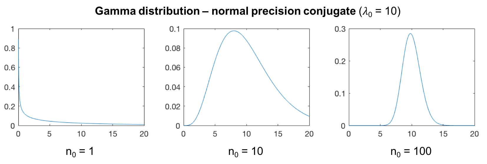
When the Gamma distribution is used as a conjugate prior for the precision parameter of a univariate Normal distribution, it is easier to parameterise it in terms of its expected value, $\lambda_0$, and degrees of freedom, $n_0$:

$$\begin{align*} \mathcal{G}_\mathcal{N}\left(\lambda_0, n_0\right) & = \mathcal{G}\left(\frac{n_0}{2}, \frac{n_0}{2\lambda_0}\right) \\ \mathbb{E}\left[\lambda\right] & = \lambda_0 \\ \mathbb{E}\left[\ln \lambda\right] & = \ln\lambda_0 + \psi\left(\frac{n_0}{2}\right) - \ln\frac{n_0}{2} \\ \mathbb{V}\left[\lambda\right] & = \frac{n_0}{2}\lambda_0^2 \\ \mathbb{V}\left[\ln \lambda\right] & = \psi_1\left(\frac{n_0}{2}\right) \end{align*}$$

The distribution has a mode only if $n_0 \geqslant 2$:

$$\max_\lambda \mathcal{G}_\mathcal{N}\left(\lambda \mid \lambda_0, n_0\right) = \lambda_0\frac{n_0-2}{n_0}$$

KL-divergence

$$\boxed{\begin{split}\mathrm{KL}\left(\lambda_1, n_1 \middle\| \lambda_0, n_0\right) ={} & -\frac{n_0}{2}\ln\frac{n_0\lambda_1}{n_1\lambda_0} + \frac{n_1}{2}\left(\frac{n_0\lambda_1}{n_1\lambda_0} - 1\right) \\ & + \ln\Gamma\left(\frac{n_0}{2}\right) - \ln\Gamma\left(\frac{n_1}{2}\right) + \frac{n_1-n_0}{2}\psi\left(\frac{n_1}{2}\right)\end{split}}$$

Parameter equivalence

$\alpha$	$\frac{n}{2}$
$\beta$	$\frac{n}{2\lambda}$
$n$	$2\alpha$
$\lambda$	$\frac{\alpha}{\beta}$

“Multivariate Normal precision scale conjugate” parameterisation

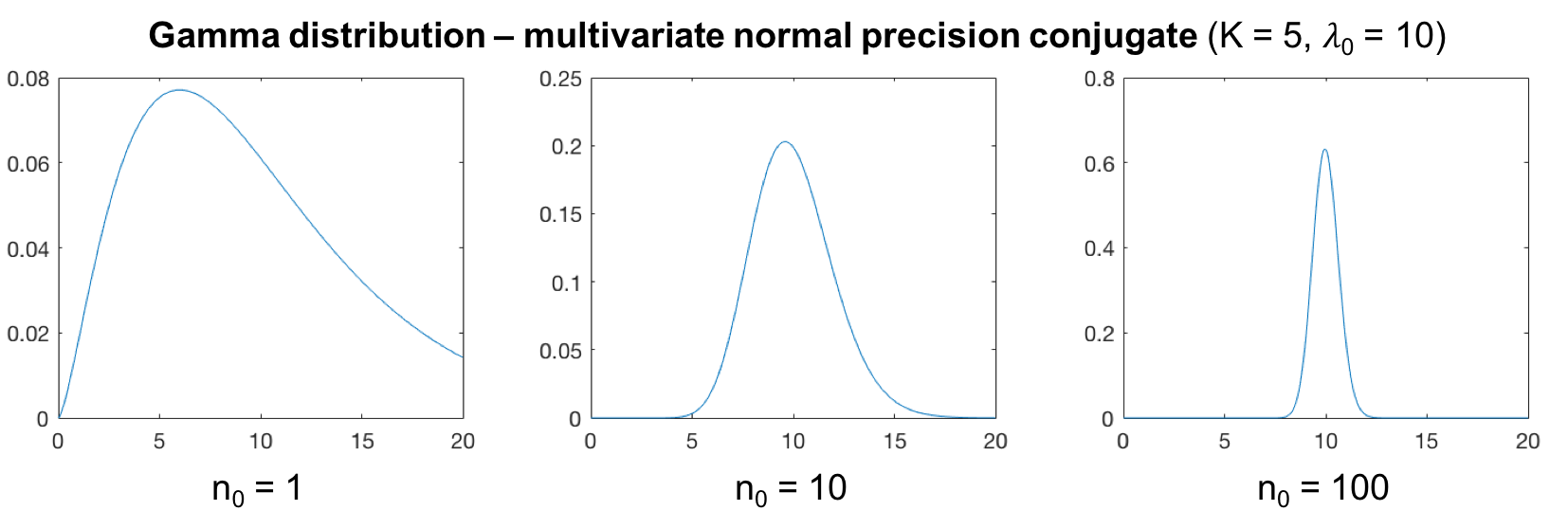
When the Gamma distribution is used as a conjugate prior for the scale of the precision matrix of a multivariate Normal distribution, it is easier to parameterise it in terms of its expected value, $\lambda_0$, and degrees of freedom, $n_0$:

$$\begin{align*} \mathcal{G}_{\mathcal{N}_K}\left(\lambda_0, n_0\right) & = \mathcal{G}\left(\frac{n_0K}{2}, \frac{n_0K}{2\lambda_0}\right)\\ \mathbb{E}\left[\lambda\right] & = \lambda_0 \\ \mathbb{E}\left[\ln \lambda\right] & = \ln\lambda_0 + \psi\left(\frac{n_0K}{2}\right) - \ln\frac{n_0K}{2} \\ \mathbb{V}\left[\lambda\right] & = \frac{n_0K}{2}\lambda_0^2 \\ \mathbb{V}\left[\ln \lambda\right] & = \psi_1\left(\frac{n_0K}{2}\right) \end{align*}$$

Note that the “Univariate Normal precision conjugate” is a spacial case of this distribution with $K = 1$.

The distribution has a mode only if $n_0 \geqslant \frac{2}{K}$:

$$\max_\lambda \mathcal{G}_{\mathcal{N}_K}\left(\lambda \mid \lambda_0, n_0\right) = \lambda_0\frac{n_0 - \frac{2}{K}}{n_0}$$

KL-divergence

$$\boxed{\begin{split} \mathrm{KL}\left(\lambda_1, n_1 \middle\| \lambda_0, n_0\right) ={} & \frac{K n_0}{2}\ln\frac{n_0\lambda_1}{n_1\lambda_0} + \frac{K n_1}{2}\left(1 - \frac{n_0\lambda_1}{n_1\lambda_0}\right) \\ & + \ln\Gamma\left(\frac{K n_1}{2}\right) - \ln\Gamma\left(\frac{K n_0}{2}\right) - \frac{K(n_1-n_0)}{2}\psi\left(\frac{K n_1}{2}\right) \end{split}}$$

Parameter equivalence

$\alpha$	$\frac{nK}{2}$
$\beta$	$\frac{nK}{2\lambda}$
$n$	$\frac{2\alpha}{K}$
$\lambda$	$\frac{\alpha}{\beta}$

“Gamma rate” parameterisation

When the Gamma distribution is used as a conjugate prior for the rate parameter of another Gamma distribution, it is easier to parameterise it in terms of its expected value, $\beta_0$, and degrees of freedom, $n_0$:

$$\begin{align*} \mathcal{G}_\alpha\left(\beta_0, n_0\right) & = \mathcal{G}\left(n_0\alpha, \frac{n_0\alpha}{\beta_0}\right) \\ \mathbb{E}\left[\beta\right] & = \beta_0 \\ \mathbb{E}\left[\ln \beta\right] & = \ln\beta_0 + \psi\left(n_0\alpha\right) - \ln n_0\alpha \\ \mathbb{V}\left[\beta\right] & = n_0\alpha\beta_0^2 \\ \mathbb{V}\left[\ln \beta\right] & = \psi_1\left(n_0\alpha\right) \end{align*}$$

The distribution has a mode only if $n_0 \geqslant \frac{1}{\alpha}$:

$$\max_\lambda \mathcal{G}_\alpha\left(\beta \mid \beta_0, n_0\right) = \beta_0\frac{n_0-\frac{1}{\alpha}}{n_0}$$

Parameter equivalence

$\alpha$	$n_0\hat{\alpha}$
$\beta$	$\frac{n_0\hat{\alpha}}{\beta_0}$
$n_0$	$\frac{\alpha}{\hat{\alpha}}$
$\beta_0$	$\frac{\alpha}{\beta}$

---

Created by Yaël Balbastre on 9 April 2018. Last edited on 10 April 2018.

---