Scaling tissue probability maps

Context

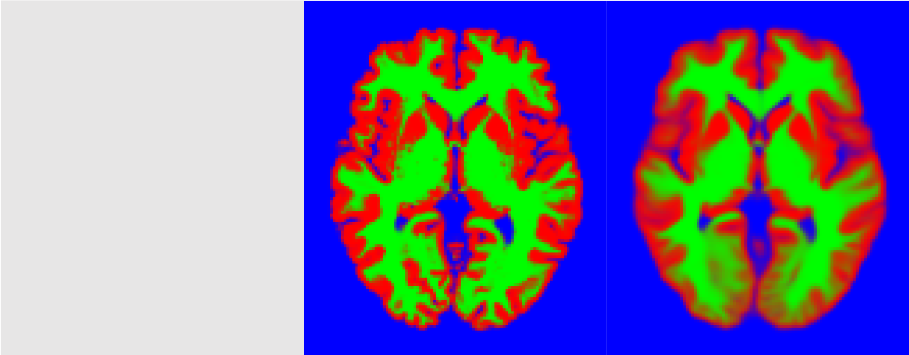
Tissue probability maps (TPMs), or templates, encode the prior probability of each voxel in an image of belonging to one of $K$ classes. Typically, they reflect the proportion of subjects, in the general population, that show a given class in a given location. These TPMs play a crucial role in segmentation models as they provide local prior information about class probability, thus helping regularise the segmentation in an anatomical way. TPMs are aligned to each observed brain and deformed to match as well as possible their anatomy¹. The following figure shows a brain image along with the true labels and the deformed template (each color represents one class, mixed colors correspond to class probabilities):

True labels and template — **Figure 1.** A brain MR image, the corresponding true labels and the warped TPMs.

In the best case scenario, the deformed TPMs would match almost exactly the true labels. However, because deformations are not entirely free (i.e., they must be smooth), there is often some kind of leeway, especially if the observed image possess an unusual anatomy (as might be the case if it is pathological). In this case, an issue is that the global expected class proportions in the template might be different from the actual class proportion, and thus bias the segmentation. In the above exemple, the expected tissue proportions, are [0.21 0.19 0.60] whereas the true proportion is [0.21 0.20 0.59]. Consequently, it is necessary to modulate the TPMs to change the global expected class proportion.

When is it useful?

When the alignement procedure has low flexibility. Typically, if only an affine transform is used, there is no chance that it may compensate for differences in gray matter volume. In this case, it is important to rescale the TPMs to avoid biasing the segmentation.
When the subject is very pathological. In this case, even with a very flexible deformation model (such as diffeomorphisms), it is possible that TPMs cannot match the subject well enough, and thus that expected proportions are not perfectly suited.

Formal writing

Let us write the true labels as a series of binary images, each acting as a mask of voxels belonging to one class. In vector form, this yields: $\mathbf{z} = \left[z_i^{(k)} \in \left\{0,1\right\} \mid i \in 1\dots I ~;~ k \in 1\dots K \right]$, where $i$ indexes voxels and $k$ indexes classes. In a similar fashion, we write the template as a series of probability images: $\boldsymbol{\mu} = \left[\mu_i^{(k)} \in \left[0,1\right] \mid i \in 1\dots I ~;~ k \in 1\dots K \right]$. The idea is to find a series of factors, $w_k$, so that prior probabilities become²:

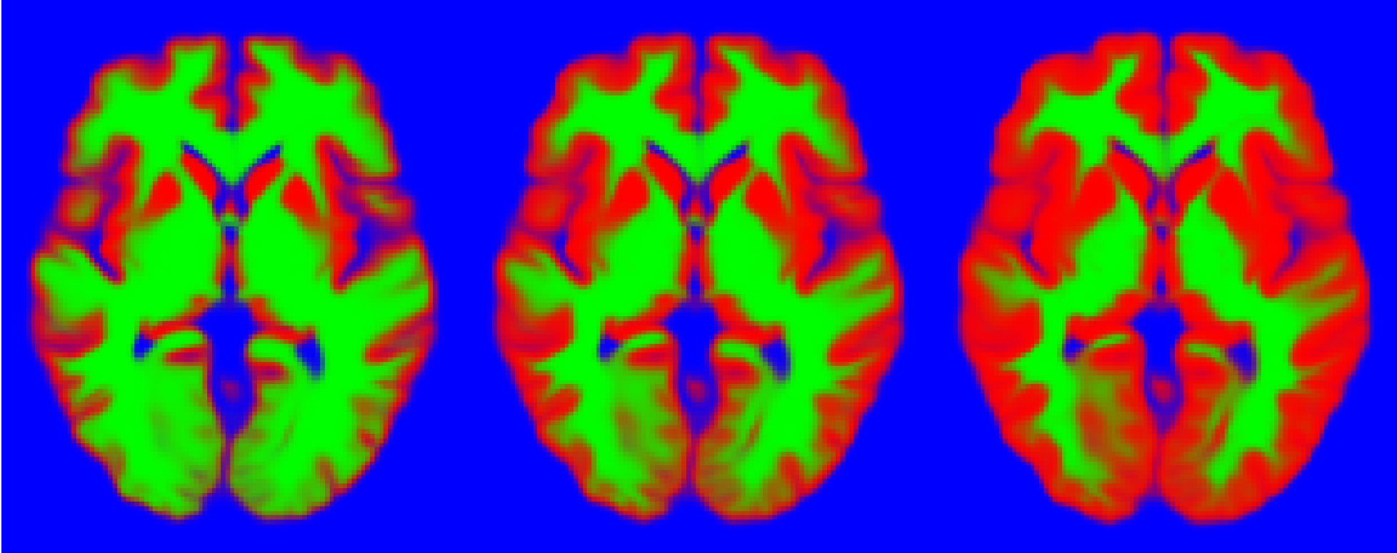
$p_i^{(k)} = \frac{w_k\mu_i^{(k)}}{\sum_{l=1}^K w_l\mu_i^{(l)}} \Leftrightarrow \mathbf{p}_i = \mathrm{pnorm}\left(\mathrm{diag}(\mathbf{w}) \boldsymbol{\mu}_i\right)$

Here, we denote by pnorm the function that normalises discrete “probabilities”. The following figure shows the above template modulated using different factors. It is apparent that each one bears very different prior information.

Rescaled templates by 3 different factors. — **Figure 2.** Rescaling by three different factors that modulate the ammount of grey and white matter in the brain.

Formally, saying that these are probabilities of belonging to each class is equivalent to saying that they are parameters of a Categorical distribution, from which stem the actual labels. We can thus write the conditonal probability:

$\forall i \in 1\dots I,~ p(\mathbf{z}_i \mid \boldsymbol{\mu}_i, \boldsymbol{w}) = \mathcal{C}\left(\mathbf{z}_i ~\middle|~ \mathbf{p}_i \right) = \prod_{k=1}^K \left(p_i^{(k)}\right)^{z_i^{(k)}}$

The conditional log-likelihood of the complete image can be written as:

$\begin{split}\mathcal{L} & = \sum_{i=1}^I \sum_{k=1}^K \left[ z_i^{(k)}\left(\ln w_k + \ln \mu_i^{(k)} - \ln\left(\sum_{l=1}^Kw_l\mu_i^{(l)}\right)\right) \right] \\ & = \sum_{k=1}^K \left[ \left(\sum_{i=1}^I z_i^{(k)}\right)\ln w_k + \sum_{i=1}^I z_i^{(k)} \ln\mu_i^{(k)} \right] - \sum_{i=1}^I \left[ \left(\sum_{k=1}^K z_i^{(k)}\right) \ln\left(\sum_{l=1}^Kw_l\mu_i^{(l)}\right) \right] \end{split}$

Maximum likelhood

A first strategy is to find a maximum likelihood (ML) value for the weights, that is, the value that maximises the conditional log-likelihood³:

$\hat{\mathbf{w}} = \arg\!\min_{\mathbf{w}} -\sum_{i=1}^I \ln p(\mathbf{z}_i \mid \boldsymbol{\mu}_i, \boldsymbol{w})$

Differentiating with respect to the weights yield:

$\mathbf{g} = \sum_{i=1}^I \left(\sum_{k=1}^K z_i^{(k)}\right) \frac{\boldsymbol{\mu}_i}{\mathbf{w}^{\mathrm{T}}\boldsymbol{\mu}_i} - \mathrm{diag}(\mathbf{w})^{-1}\left(\sum_{i=1}^I\mathbf{z}_i\right)$

Sadly, this gradient cannot be solved in closed form. A first solution, used in Ashburner’s Unified Segmentation (Ashburner and Friston, 2005), is to assume $\boldsymbol{\mu}_i^{\mathrm{T}} \mathbf{w}$ constant (i.e., it keeps a previous value), yielding:

$\tilde{\mathbf{w}} = \mathrm{diag}\left(\sum_{i=1}^I\mathbf{z}_i\right)^{-1}\left(\sum_{i=1}^I \left(\sum_{k=1}^K z_i^{(k)}\right) \frac{\boldsymbol{\mu}_i}{\mathbf{w}^{\mathrm{T}}\boldsymbol{\mu}_i}\right)$

A second solution is to obtain the optimum numerically with a Gauss-Newton optimisation scheme. In this case, we also need the second derivatives of the objective function:

$\mathbf{H} = \mathrm{diag}\left(\mathrm{diag}(\mathbf{w})^{-2}\left(\sum_{i=1}^I\mathbf{z}_i\right)\right) - \sum_{i=1}^I \left(\sum_{k=1}^K z_i^{(k)}\right) \frac{\boldsymbol{\mu}_i \boldsymbol{\mu}_i^{\mathrm{T}}}{\left(\mathbf{w}^{\mathrm{T}}\boldsymbol{\mu}_i\right)^2}$

The optimum can then be optained iteratively, according to the update scheme:

$\mathbf{w}^{(n+1)} = \mathbf{w}^{(n)} - \left[\mathbf{H}^{(n)}\right]^{-1} \mathbf{g}^{(n)}$

Since $w_k \in \mathbb{R}^+$, it might be better to define it as $w_k = \exp(\gamma_k)$. The corresponding gradient and Hessian are provided below:

$\mathbf{g} = \left(\sum_{i=1}^I \left(\sum_{k=1}^K z_i^{(k)}\right) \frac{\mathrm{diag}(\mathbf{w})\boldsymbol{\mu}_i}{\mathbf{w}^{\mathrm{T}}\boldsymbol{\mu}_i}\right) - \left(\sum_{i=1}^I \mathbf{z}_i\right)$ $\mathbf{H} = \left(\sum_{i=1}^I \left(\sum_{k=1}^K z_i^{(k)}\right) \frac{\mathrm{diag}\left(\mathrm{diag}(\mathbf{w})\boldsymbol{\mu}_i\right)}{\mathbf{w}^{\mathrm{T}}\boldsymbol{\mu}_i}\right) - \sum_{i=1}^I \left(\sum_{k=1}^K z_i^{(k)}\right) \frac{\mathrm{diag}(\mathbf{w})\boldsymbol{\mu}_i \boldsymbol{\mu}_i^{\mathrm{T}}\mathrm{diag}(\mathbf{w})}{\left(\mathbf{w}^{\mathrm{T}}\boldsymbol{\mu}_i\right)^2}$ $\mathbf{w}^{(n+1)} = \mathrm{diag}\left(\exp\left(\left[\mathbf{H}^{(n)}\right]^{-1} \mathbf{g}^{(n)}\right)\right)^{-1}\mathbf{w}^{(n)}$

Derivatives were obtained with Matlab’s symbolic toolbox as expained here.

Conjugate prior

Let’s try to find a prior probability distribution on the weights that would make the posterior distribution tractable. First, it needs to be defined on $\mathbb{R}^+$. Second, by applying Bayes’ rule, the posterior can be written as:

$p(\mathbf{w} \mid \mathbf{z}, \boldsymbol{\mu}) \propto p(\mathbf{z}, \mid \mathbf{w}, \boldsymbol{\mu}) p(\mathbf{w} \mid \boldsymbol{\mu})$

Note than we have used $\boldsymbol{\mu}$ as a parameter throughout. Consequently, a conjugate prior would have the same functional form with respect to $\mathbf{w}$ as the conditional probability, i.e.:

$\ln p(\mathbf{w} \mid \boldsymbol{\mu}) \overset{c}{=} \sum_{k=1}^K \gamma_k \ln w_k - \sum_i \beta_i \ln\left(\sum_{k=1}^K w_k \mu_i^{(k)}\right)$

Let’s now write a function of $\mathbf{w}$ that “corresponds” to placing a Dirichlet prior on each reconstructed voxel, i.e.:

$\begin{split} f(\mathbf{w}) & = \sum_{i=1}^I \ln\mathcal{D}\left(\mathrm{pnorm}(\mathrm{diag}(\mathbf{w}) \boldsymbol{\mu}_i) \mid \boldsymbol{\alpha}_i\right) \\ & \overset{c}{=} \sum_{k=1}^K \left[ \left(\sum_{i=1}^I \left(\alpha_i^{(k)}-1\right)\right)\ln w_k + \sum_{i=1}^I \left(\alpha_i^{(k)}-1\right) \ln\mu_i^{(k)} \right] \\ & \phantom{=} - \sum_{i=1}^I \left[ \left(\sum_{k=1}^K \left(\alpha_i^{(k)}-1\right)\right) \ln\left(\sum_{l=1}^Kw_l\mu_i^{(l)}\right) \right] \end{split}$

We recognise exactly the same form as the conditional likelihood. An important question, however, is to known if this function can be used to define a probability distribution on $\mathbf{w}$. In other words, is $\int_{\mathbb{R}^+} \exp(f(\mathbf{w})) \mathrm{d}\mathbf{w}$ finite? The problem is that the function that maps $\mathbf{w}$ to $\mathrm{pnorm}(\mathrm{diag}(\mathbf{w}) \boldsymbol{\mu}_i)$ is surjective, since for any factor $a$,

$\mathrm{pnorm}(a \cdot \mathrm{diag}(\mathbf{w}) \boldsymbol{\mu}_i) = \mathrm{pnorm}(\mathrm{diag}(\mathbf{w}) \boldsymbol{\mu}_i)$

We will assume anyway that the above function allows defining a probability distribution. What value should we choose for its parameters $\mathbf{\alpha}_i$? When no other information is known, it is rational to think that the observed image stems from the same population as the template, and as such, that:

$\mathbb{E}\left[\mathrm{pnorm}(\mathrm{diag}(\mathbf{w}) \boldsymbol{\mu}_i)\right] = \boldsymbol{\mu}_i$

This gives us the weight repartition between the different classes, i.e., $\boldsymbol{\alpha}_i \propto \boldsymbol{\mu}_i$. The missing factor is an indicator of how confident we should be in the prior. If it is near zero, the observations will have a lot of power ; if it is very large, the prior will have a lot of power. This can be an user-defined value, that we will name $n$. Two values make sense: 1 (to give as much weight to the data and to the template) and $N$, the number of subjects that were used to build the template.

Posterior

Thanks to the conjugate prior, we can easily write the log-posterior probability as:

$\begin{split}\ln p(\mathbf{w} \mid \mathbf{z}, \boldsymbol{\mu}, n) \overset{c}{=} & \sum_{k=1}^K \left[ \left(\sum_{i=1}^I \left(z_i^{(k)} + n\mu_i^{(k)}-1\right)\right)\ln w_k \right] \\ & - \sum_{i=1}^I \left[ \left(\sum_{k=1}^K \left(z_i^{(k)} + n\mu_i^{(k)}-1\right)\right) \ln\left(\sum_{l=1}^Kw_l\mu_i^{(l)}\right) \right] \end{split}$

Maximum a posteriori

A MAP estimate can be obtained with the same methods as the ML estimate, since both objective functions have the same form. The only difference is that there might be some (hopefully very rare) cases where the posterior does not possess a mode. The expected value of our distribution being intractable, we have no choice but to resolve to a mode estimate.

Created by Yaël Balbastre on 27 March 2018. Last edited on 29 March 2018.

We do not tackle the issue of deforming TPMs in this article. It may be done beforehand or, more consistantly, at the same time as the segmentation in an iterative fashion. ↩
In this article, we will often use $\mathrm{diag}(\mathbf{a})\mathbf{b} = [a_k b_k]_{k = 1 \dots K}$ to indicate an element-wise (or Hadamard) product between two vectors. ↩
Using the log-likelihood rather than the likelihood has several advantages. First, because the logarithm is strictly monotonic, a maximum of the log-likelihood is a maximum of the likelihood. Second, it transforms products in sums, often easing the differentiation. Third, it is a transform that is used to solve problems with hidden variables, along with the Expectation-Maximisation algorithm, because of its concavity. ↩

Computational Anatomy notes